
Comprehensive Guide to the Nichols-Ziegler PID Tuning Method
Look—if you’ve ever stared at a process loop that won’t settle, or watched an output bounce around like a hyperactive toddler, you’ve probably heard the name Ziegler-Nichols thrown around. But let’s talk about the less famous cousin: the Nichols-Ziegler PID tuning method. I’ve spent over a decade tuning loops in everything from chemical reactors to HVAC systems, and I can tell you this: understanding this method is like having a cheat code for stable, responsive control. And unlike some modern “auto-tune” black boxes, this approach actually makes you think. Seriously, it forces you to understand your process. That’s a good thing.
The Nichols-Ziegler PID tuning method (sometimes called the ultimate sensitivity method) was developed back in the 1940s by two engineers who clearly had better things to do than write boring manuals. They wanted a systematic way to find PID gains without endless trial and error. The core idea? Find the point where your loop starts to oscillate—the ultimate gain and ultimate period—and then back off with some very specific formulas. It’s a big deal because it works for a huge range of processes, from slow temperature loops to fast pressure systems. Honestly, I’ve used it on everything except maybe my coffee maker (though I’m tempted).
Now, I’ll walk you through the entire process—from theory to hands-on execution—with the kind of practical depth you’d expect from someone who’s been elbow-deep in tuning panels for years. No fluff. No corporate-speak. Let’s dive in.
---
How the Nichols-Ziegler Method Actually Works (No Magic Here)
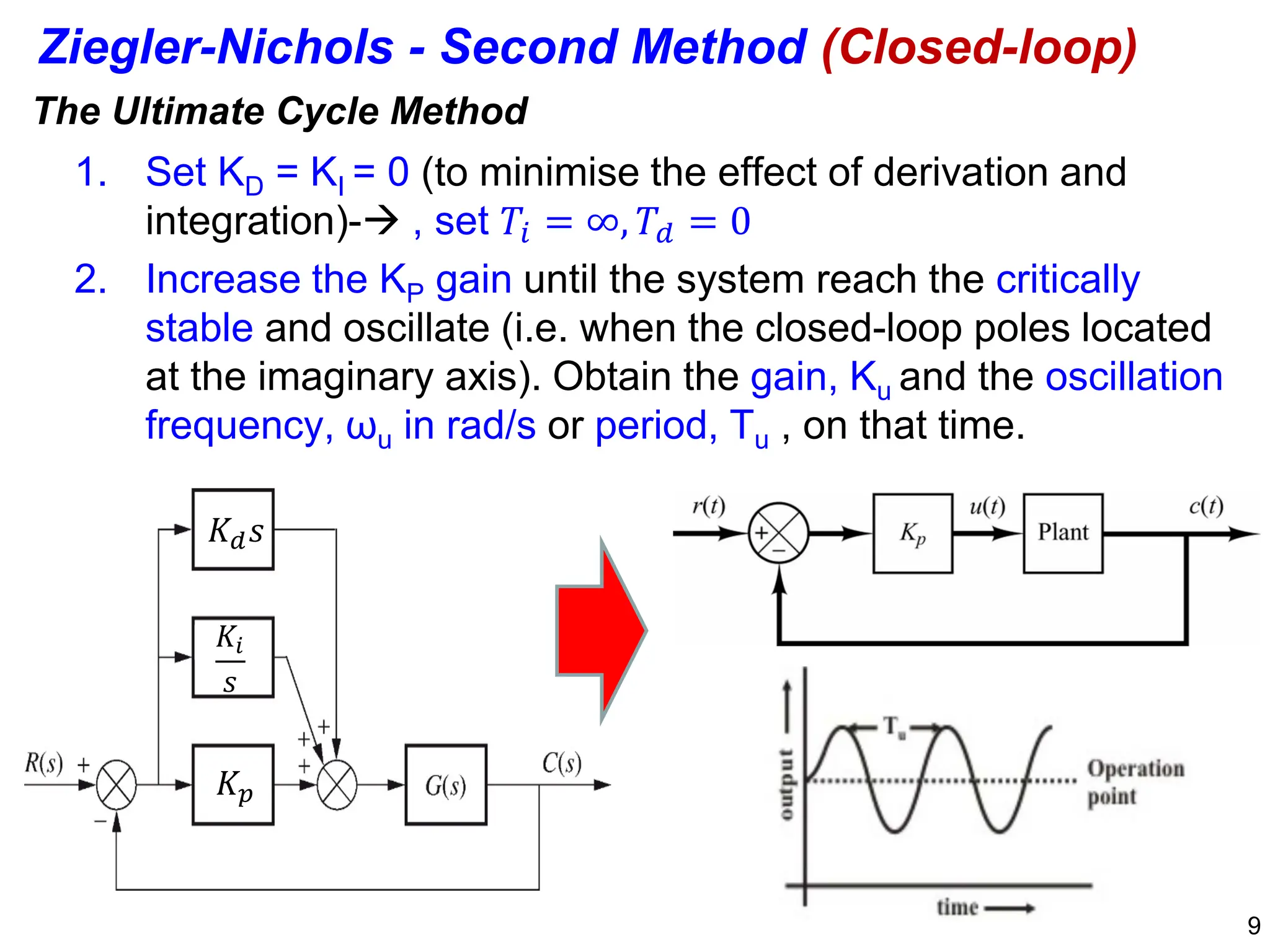
The principle is deceptively simple: you force your control loop into sustained oscillations by cranking up the proportional gain until you hit a critical point. Then you measure two key parameters: the ultimate gain (Ku) and the ultimate period (Pu). From there, the Nichols-Ziegler PID tuning method gives you a set of equations to calculate P, I, and D gains that produce a 1/4 amplitude decay ratio. In plain English? You want the overshoot to shrink by three-quarters every cycle. It’s a classic trade-off between responsiveness and stability.
Let me be blunt—this method assumes your process can handle being pushed into oscillation without causing a disaster. If you’re tuning a nuclear reactor coolant loop, maybe skip this and call an expert. For most industrial processes, though, it’s safe if you perform the test carefully. I’ve seen operators freak out when the output starts cycling. Relax. That’s the point.
The Ultimate Gain Experiment: Step-by-Step
Before you start, make sure your controller is in automatic mode and all integral and derivative actions are turned off (I=0, D=0). Set the proportional band to a safe value—like 5 or 10% gain (which is a low gain). Then introduce a small setpoint change. If the response is sluggish, increase the proportional gain. Keep doing this with tiny bumps. What you’re looking for is the onset of constant-amplitude oscillations. The gain at which those oscillations become sustained and uniform is your ultimate gain (Ku). The time between peaks is your ultimate period (Pu).
Here’s the tricky part: you need to distinguish between a real ultimate oscillation and a noisy process signal. I’ve seen people mistake a random bump for a cycle. Pro tip: let the oscillation run for at least 3-4 full cycles. If the amplitude stays constant (within reason), you’ve found it. If it’s growing or decaying, you’re not there yet. Write down Ku and Pu. Seriously, scribble them on a scrap of paper. You’ll need them in the next step.
Why Sustained Oscillations? (And When It’s a Bad Idea)
The beauty of sustained oscillations is they reveal the natural dynamics of your process at the stability boundary. The Nichols-Ziegler PID tuning method exploits this to give you gains that are mathematically derived from a second-order model approximation. But here’s the catch: not all processes can handle full oscillation. Fast loops (like pressure or flow) can oscillate at frequencies that damage valves or cause cavitation. Slow loops (temperature, level) are usually safer. Use your judgment. If you’re tuning a loop that controls a knife-edge process, consider a different method—like the Cohen-Coon or a simple trial-and-error approach.
I recall tuning a large industrial oven once. The ultimate period was over 20 minutes. Watching that oscillation was like watching paint dry, but it worked. The final PID settings gave me rock-solid temperature control. So yes, patience is a virtue.
---
Crunching the Numbers: Nichols-Ziegler Formulas for P, PI, PID
Once you have your Ku and Pu, the math is straightforward. The Nichols-Ziegler PID tuning method provides different formulas depending on the controller type you want to use. Here’s the classic set (note: these are for the “standard” form, not the “parallel” form—check your controller documentation):
- P-only controller: Kp = 0.5 * Ku
- PI controller: Kp = 0.45 * Ku, Ti = Pu / 1.2
- PID controller: Kp = 0.6 * Ku, Ti = Pu / 2, Td = Pu / 8
Yes, it’s that simple. But don’t let the simplicity fool you. These gains are a starting point, not a final answer. I’ve seen engineers plug them in and walk away, only to come back to a loop that oscillates annoyingly. The 1/4 decay ratio is an aggressive target. If your process demands no overshoot at all (like a pharmaceutical reactor), you should reduce the gains—say, start with 0.3 * Ku for proportional. Always test.
What About Integral and Derivative Units?
One common gotcha: the formulas above give Ti (integral time) and Td (derivative time) in minutes or seconds, depending on your ultimate period unit. If you measured Pu in seconds, then Ti is in seconds. If your controller uses “reset rate” (repeats per minute) instead of time, you’ll need to convert: reset rate = 60 / Ti. Derivative rate (minutes) is the same as Td. I’ve lost count of how many times I’ve seen someone put in a derivative time of 8 seconds when it should have been 0.5 seconds. Double-check your controller’s unit convention. It’s a big deal.
Another nuance: the Nichols-Ziegler PID tuning method was designed for analog controllers. Digital controllers sometimes behave differently due to sampling time. If your controller updates slowly (say, once per second), derivative action can become noisy. In that case, consider using a PI controller instead, or apply a derivative filter. Honestly, 90% of my loops run fine with just PI. Derivative is a spice—use it sparingly.
Adjusting for Process Non-Linearities
No process is perfectly linear. The ultimate gain you found at one operating point might change if the load shifts. I always recommend verifying the tuning at a couple of different conditions. If the loop starts ringing at a different load, your gains are likely too high. The Nichols-Ziegler PID tuning method assumes a linear process around the test point. In practice, you’ll often need to apply a safety factor: multiply Ku by 0.4 for the PID gain instead of 0.6 if your process has significant dead time. Use your gut. That’s the “expert specialist” part.
---
Common Pitfalls (And How to Avoid Making a Fool of Yourself)
I’ve coached dozens of engineers through this method, and I keep seeing the same mistakes. Let me save you some embarrassment.
- Starting with integral action on. If you leave any integral in your controller during the test, it will integrate the error and prevent sustained oscillations. You’ll never find the true Ku. Turn it off completely.
- Confusing ultimate period with process time constant. The ultimate period is the oscillation period at the stability limit, not the open-loop time constant. They’re related but different. Don’t mix them.
- Using too large a setpoint bump. A small bump (like 1-2% of range) is enough. Big bumps can saturate the output or trigger alarms. Think gentle, not violent.
- Ignoring measurement noise. If your signal is noisy, the oscillation may be hard to detect. Add a small filter (like a 1-second time constant) before the test, but note that filtering affects the ultimate period. Compensate by subtracting the filter time constant from Pu if needed.
- Not testing at the worst-case load. The loop might behave differently near extremes. Test at low load and high load if possible.
One time, a junior engineer set the proportional gain to 200% on a flow loop without verifying the valve limits. The output slammed from 0 to 100% in one cycle. The valve actuator nearly failed. Learn from his mistake—check your limits first.
When the Nichols-Ziegler Method Fails (And What to Do Instead)
It’s rare, but sometimes the method just doesn’t work. This happens when: - The process has dominant dead time (like a long transport delay). The oscillation becomes very slow and the gains you get are too aggressive. - The process is integrating (like a tank level without outflow). Sustained oscillations may not be achievable because the process integrates the error. - The process has significant nonlinearities or hysteresis.
In those cases, I fall back on alternative tuning methods: lambda tuning for dead time, or the IMC-based method for integrating processes. But for 70% of common loops—temperature, pressure, simple flow—the Nichols-Ziegler PID tuning method is your best friend.
---
Common Questions About the Nichols-Ziegler PID Tuning Method
Q: Is the Nichols-Ziegler method the same as the Ziegler-Nichols method?
Technically, yes—the Nichols-Ziegler method is often called the Ziegler-Nichols ultimate sensitivity method. The two engineers collaborated on both the process reaction curve method and this one. But in practice, the term “Nichols-Ziegler” specifically refers to the closed-loop oscillation tuning approach. It’s a semantic difference. You’ll hear both names.
Q: Can I use this method on a loop that already has some tuning?
Absolutely. Just set your existing PID gains to zero for I and D, and set the proportional gain to a low value. Then perform the test as described. The existing P gain won’t interfere as long as you start low and increase it. Just be aware that the ultimate gain you find may be different from a completely naked loop because the controller’s own internal settings can affect the dynamics slightly. It’s fine for practical use.
Q: What if I can’t achieve sustained oscillations?
If the output never stabilizes into constant amplitude—either it grows uncontrollably or decays immediately—you’re likely in a region where the process is not amenable to this method. Try reducing the proportional gain further and using a larger setpoint change. If it still doesn’t work, your process may be highly nonlinear or have excessive dead time. Consider the open-loop method (process reaction curve) instead.
Q: How often should I re-tune using the Nichols-Ziegler method?
Only when the process changes. If your system is well maintained and the dynamics are stable (say, a water temperature loop with the same piping), you might never need to retune. But if you add new equipment, change setpoints significantly, or notice oscillations, run the test again. As a rule of thumb, check once a year or after any major maintenance.
Q: Is this method safe for critical loops like pressure or flow?
It can be risky because oscillations at high frequency can damage actuators or cause process upsets. For critical loops, I recommend a bump test (open-loop step response) instead. Or use a very small gain increment and monitor closely. When in doubt, consult a senior engineer. Safety first.
---
Let me leave you with this: the Nichols-Ziegler PID tuning method is one of the most powerful tools in a control engineer’s toolbox, but it’s not a magic wand. It gives you a great starting point, but you still need to verify and adjust based on your process’s personality. I’ve seen perfect-looking calculations lead to lousy performance because the engineer ignored valve hysteresis or sensor lag. So go ahead, run the test, crunch the numbers, but watch your loop like a hawk during the first few setpoint changes. That hands-on feel is something no formula can replace.