
The Histogram Won't Lie: A Tutorial on Optimizing Bin Width for Accurate Data Counts
Ever stared at a histogram and felt like it was lying to you? Seriously. I've been there. You look at a distribution, and your data either looks like a perfectly smooth bell curve or a jagged mess that makes no sense. The culprit isn't your data. It's your bin width. You can have the cleanest dataset on the planet, but if you screw up the bins, your accurate data counts are toast. I've spent over a decade cleaning up messes made by automatic plotting software defaults. This tutorial on optimizing bin width is the fix. We're going to get this right.
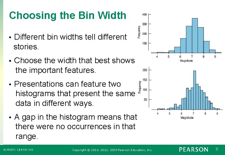
Think of your histogram like a pair of binoculars. Turn the focus wheel too far one way, and everything blurs together. Too far the other way, and you see individual dust specks on the lens but miss the mountain. The bin width is that focus wheel. It determines how we group raw numbers into columns. Get it wrong, and you either hide the story your data is trying to tell, or you invent noise that isn't there. This isn't just academic. It's about making real decisions based on real numbers.
Most people just hit 'default' in Excel or Python. That's a trap. Defaults are designed for generic situations. Your data isn't generic. It's specific. It's gnarly. It's full of personality. If you treat every dataset the same way, you're going to get misleading data distribution visuals. And misleading visuals lead to bad conclusions. Trust me, I've seen a CEO make a million-dollar decision based on a poorly binned histogram. Don't let that be you.
The goal here is simple: to give you the tools to build a histogram that's honest. We'll cover the math, but more importantly, the logic behind the math. By the end, you'll know how to pick a histogram bin width that actually reflects your underlying data frequency without distorting the truth. Let's dive into the core problem first.
The Golden Rule: Why Your Bin Width Matters More Than You Think
This isn't a 'nice to have' skill. It's the difference between a chart that communicates and a chart that confuses. I remember a project where a client was convinced their manufacturing process had two separate defects. The default histogram showed two distinct peaks. Looked clear as day. I dug deeper. The bin width was too small. It was splitting a single, slightly skewed distribution into two false peaks. We adjusted the width, and the bimodal illusion vanished. We saved them weeks of pointless troubleshooting. That's the power of optimizing bin width.
When you're working with accurate data counts, the bin width directly controls the resolution. Too many bins (too narrow), and you're chasing statistical ghosts. Each bin has only a couple of data points. The pattern looks like a broken comb. You can't see the forest for the trees. Too few bins (too wide), and you're hiding all the interesting details. Everything gets thrown into massive buckets. You lose the peaks, the valleys, the outliers. You get a blocky, uninspired shape that tells you almost nothing.
There's a concept in statistics called the bias-variance tradeoff. It applies perfectly here. A narrow bin width gives you high variance (the chart looks wild and jumpy). A wide bin width gives you high bias (the chart is smooth but potentially wrong). Your job is to find the sweet spot in the middle. Look—every dataset has an optimal data binning strategy. It's not magic. It's math. But it's math you can understand.
Let's break down the two classic mistakes you'll encounter. Knowing these is half the battle.
The Squeeze: What Happens When Bins Are Too Small
I call this the 'Chia Pet' histogram. It looks fuzzy. It looks organic. It looks like scared noise. When you set your histogram bin width too small, every single data point tries to become its own column. The result is a jagged, spiky mess. The spikes are random. They aren't telling you about your data distribution. They're telling you about the luck of the draw in your sampling. You lose the signal in the noise.
Honestly? This is the most common mistake I see from people who think they are being 'precise.' They think smaller bins mean more detail. They're wrong. More detail isn't always better. If I zoom in on a pixel of a photograph, I don't see the picture. I see a square. That's what narrow bins do to your data. They break the picture into meaningless squares. Your accurate data counts become an illusion of precision.
The math behind this is simple. If your bin width is less than the typical distance between similar data points, you're artificially creating gaps. Real continuous data shouldn't have huge cliffs between adjacent bins. If it does, you're probably overfitting the visualization. Your eye starts to see patterns in the randomness. We're wired for that. Don't let your brain fool you. The chart should look smoothish, not like a picket fence.
A good rule of thumb I use in practice: if your histogram looks 'fragile,' like a slight change in the data source would change the shape dramatically, the bin width is probably too small. Recalculate it. Your distribution should be stable. It should pass the 'nudge test' — if you add or remove a few data points, the shape shouldn't collapse into something completely different.
The Smear: The Danger of Overly Wide Bins
On the opposite end, we have the 'Smear.' This is when you use a bin width that's way too big. Everything gets lumped into one or two massive buckets. This is the classic 'the data looks like a brick' histogram. It's useless. It hides multimodality. It conceals skewness. It buries outliers. It's a data crime, and I see it all the time in corporate slide decks. Look—if your histogram has four bars or less, you aren't doing data analytics. You're just drawing rectangles.
Think about a distribution that has two distinct populations. Maybe you have measurements from two different machines. A wide bin width will merge those two peaks into one big, fat, average-looking hump. You'll never know your process is broken. The chart will look 'normal.' It will feel 'safe.' It will be a lie. Optimizing bin width is about uncovering these hidden truths, not hiding them under a rug of aggregated data.
The problem is that wide bins inflate your data frequency counts for the middle values and deflate them for the extremes. You lose the tail behavior. In finance, the tail is where the risk is. In manufacturing, the tail is where the defects are. If you smear your data into a blob, you can't see the tail. You can't manage the risk. You can't fix the defects. The chart becomes a tool for ignorance, not insight.
So how wide is too wide? A simple test: look at the maximum and minimum values. Divide the range by the number of bins. If that number is huge (more than 10-20% of the total range), you've got a smearing problem. Your data visualization is failing you. Time to tighten the focus.
The Big Three Methods: How to Calculate Optimal Bin Width
Alright, enough horror stories. Let's get practical. Over the years, three methods have proven to be the workhorses for optimizing bin width. They aren't perfect for every situation, but they cover 90% of real-world use cases. I use them constantly. You will too. Each method makes a different assumption about your data distribution, so understanding when to use them is key.
Don't get intimidated by the formulas. I'll walk you through the logic first. The goal is to balance the number of bins against the sample size. More data? You can afford more bins. Less data? You need fewer. The methods just formalize that intuition. Think of them as guardrails, not prison walls. You can adjust from their suggestion, but they keep you out of the ditch.
Here's a quick cheat sheet of the three contenders:
- Sturges' Rule: Based on a normal distribution assumption. Works great for bell curves.
- Scott's Rule: Focuses on minimizing the variance. Good for continuous data.
- Freedman-Diaconis Rule: Robust to outliers. My personal favorite for messy data.
Each one will give you a specific number of bins. From that, you calculate the bin width by dividing your data range by that number. Simple.
Sturges' Rule: The Old-School Workhorse
This is the method that most software defaults to. It's been around since the 1920s. The formula is simple: Number of bins = log2(N) + 1, where N is your sample size. So for 100 data points, you get about 7 or 8 bins. For 1000, you get 11. It's easy. It's fast. It's also often wrong. Seriously. It assumes your data is perfectly symmetric and normal. When does that happen? Almost never.
Sturges' Rule shines when you have a classic bell curve. In that scenario, the bin width it suggests is actually quite good for showing the shape. But the moment your data distribution gets skewed, has heavy tails, or is multimodal, Sturges fails. It tends to suggest too few bins for large datasets and too many for small datasets. It's a one-size-fits-all shoe that only fits one foot.
I use Sturges as a baseline. It's the 'check engine' light. If I'm looking at a dataset I've never seen before, I'll run Sturges first. It gets me in the ballpark. Then I look at the chart and ask, 'Does this look right?' Usually, the answer is no, and I switch to a more robust method. But it's a starting point. Don't bash it. Just don't worship it.
When should you not use it? When your data has outliers. When your sample size is under 30. When you suspect multiple peaks. Basically, use it as a sanity check, not your final answer. For accurate data counts in messy real-world data, you need a different tool.
Scott's Rule: The Normal Distribution Go-To
Scott's Rule is a step up. It's more sophisticated. It uses the standard deviation of your data to calculate the bin width. The formula is: Bin width = 3.49 standard deviation N^(-1/3). Ignore the math for a second. What this does is it adapts the bin size to the spread of your data. If your data is tightly clustered, it makes narrower bins. If it's widely spread, it makes wider bins. That's smart.
This method assumes your data is approximately normal, but it's a little more forgiving than Sturges. It handles different variances much better. If you have a dataset that looks rough but is essentially unimodal (one hump), Scott's rule is a solid choice. I use it often for quality control data where the data is usually Gaussian-ish. It gives me a clean, interpretable chart without over-smoothing.
The downside? It's still sensitive to outliers. A single extreme outlier can inflate the standard deviation, causing Scott's rule to suggest a bin width that is too wide. You end up smearing the main distribution to accommodate that one weird point. That's bad. You need to clean your data first, or use a method that ignores the outliers. For data frequency analysis, one bad apple can ruin the whole barrel.
Honestly, Scott's Rule is my second choice. It's a good all-rounder. If I'm doing a quick exploratory data analytics session and I know the data is well-behaved, I use this. But for the hard stuff, the gnarly stuff, I reach for the big gun: the Freedman-Diaconis rule.
The Practical Workflow: A Hands-On Tutorial for Optimizing Bin Width
Theory is great. Execution is better. I'm going to give you a workflow that I use every single week. It doesn't require a statistics degree. It requires a calculator (or a few lines of Python or R), and some common sense. We're going to treat optimizing bin width like a science experiment. Step by step.
First, always visualize your raw data as a Q-Q plot or a simple scatter plot. This tells you about outliers and skewness before you bin anything. You can't fix a problem you don't see. Second, calculate the interquartile range (IQR). This is the range of the middle 50% of your data. It's resistant to outliers. The Freedman-Diaconis rule uses this. It's your secret weapon.
The workflow is simple:
- Sort your data and find the 25th and 75th percentiles to get your IQR.
- Calculate the Freedman-Diaconis bin width: 2 IQR N^(-1/3).
- Calculate the number of bins: Divide your data range (max - min) by that bin width. Round up.
- Build your histogram and look at it. Does it tell a story?
That's it. Four steps. If you do this, you will be in the top 5% of people who build histograms. Seriously. Most people just click 'OK.' You will be making deliberate, informed choices about your data binning. You will produce accurate data counts that you can defend.
Step 1: Assess Your Data Distribution Before You Even Think About Bins
This is the step everyone skips. They just throw the numbers into a chart. It's lazy. Look—you need to know what you're dealing with. Is your data distribution symmetric? Skewed? Bimodal? Does it have fat tails? Run a quick descriptive stats summary. Look at the mean vs. the median. If they're very different, you have skew. Skewed data hates Sturges' Rule.
If I see a dataset with a high skew, I know immediately that I need a method based on the IQR, not the standard deviation. The IQR ignores the tails. This is crucial for optimizing bin width because the tails can distort the bin calculation. You don't want your bin width to be decided by a few extreme values. You want it to be decided by the bulk of the data. The IQR gives you that.
Check for outliers visually. A simple box plot is your friend. If you have outliers, consider capping them or analyzing them separately. Don't let five weird numbers ruin the histogram for the other 995 normal ones. An outlier is a data point, yes, but it's often a symptom of a different issue. It might need its own bin, or it might need to be excluded from the main analysis. Decide before you bin.
Honestly, this assessment takes two minutes. It saves you hours of confusion. I can't stress this enough. Know your data before you slice it. You wouldn't chop vegetables without looking at them first, right? Same deal here.
Step 2: Test and Validate Your Bin Count for the Best Fit
Once you have a candidate bin width from a formula, don't stop there. Test it. Build the histogram. Then change the bin count by +/- 2. Look at the changes. If the histogram's shape is completely different, your bin width is not stable. You need to go back and check your assumptions. A robust bin width produces a histogram that doesn't change dramatically when you nudge it.
This is what I call the 'sway test.' A good histogram has a backbone. It stands firm. If you add a bin or remove a bin, the story should be the same. The peaks and valleys should stay in the same places. If they move around like a drunk skunk, your optimal bin width hasn't been found yet. Usually, this means your data has a weird structure that the standard formulas don't handle well. Consider manual binning based on domain knowledge.
For example, if you're looking at age data, bins of 5 or 10 years often make more sense than statistical bins of 7.3 years. Don't be a slave to the math. Use the math to get close, then use your brain to fine-tune. The goal is accurate data counts that communicate. A bin width of 10 years is easier for a human to understand than a bin width of 13.6 years. Round to sensible numbers if it helps the story.
Finally, look at the bin edges. Make sure they aren't cutting right through natural clusters. This is an art, not a science. You want the bins to line up with the natural breaks in the data frequency. If your data is about exam scores and you notice a pile-up at 70, don't put a bin boundary at 70. Put it at 69.5 or 70.5. This prevents splitting a natural cluster into two bins. Little tweaks like this separate the pros from the amateurs.
Common Questions About Optimizing Bin Width
What is the best bin width formula for most datasets?
For most general-purpose work, the Freedman-Diaconis rule is the safest bet. It uses the IQR, which is resistant to outliers, making it suitable for a wide range of data distribution shapes. It's not perfect for highly multimodal data, but it's a great starting point that usually outperforms Sturges or Scott for real-world, messy data.
How does bin width affect outliers in a histogram?
A histogram bin width that is too small can make outliers look like separate isolated spikes, exaggerating their importance. A width that is too large can completely hide outliers by lumping them into an adjacent bin with normal data. The key is to use a robust method like the IQR to define the width, which minimizes the influence of extreme values.
Can I use the same bin width for comparing two different datasets?
You can, but you shouldn't unless the datasets have similar spreads and sample sizes. For accurate data counts across groups, it's often better to use the same number of bins rather than the same bin width. This ensures the histograms have the same resolution and are visually comparable. However, if the ranges are vastly different, forcing the same width will distort one of the distributions.
What happens if I have fewer than 30 data points?
With small sample sizes, any bin width formula will struggle. The concept of optimizing bin width loses some meaning because you lack the data to define the shape. In this case, I recommend using a rule of thumb like the square root of N for the number of bins, or simply considering a dot plot instead of a histogram. You want to avoid over-interpreting the shape of the chart when uncertainty is high.
Is it better to have more bins or fewer bins for accuracy?
Neither is inherently better. The goal is to find the optimal bin width that minimizes the 'binning error.' More bins reduce the bias (the bins are closer to the true data) but increase the variance (more noise). Fewer bins reduce variance but increase bias. You're balancing these two. The formulas I've shown are designed to minimize this total error for your specific data analytics task.